Yesterday I was bumping into the problem of designing a bandpass active filter using op-amps. I remember, in the late ’70s, the must-have book was this one on the right.
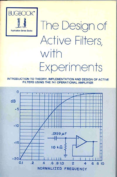
Of course I owned the Italian version and it was one of the most used books of my youth.
Nowadays that book is somewhere in my library, among thousands of other books (especially my wife’s). So I was looking for a simple utility for the PC, to aid the basic design and calculation of the most common patterns of active filters.
On the internet there are plenty of articles and utils for that, but the first one you will find is a Texas Instruments product called FilterPro. It is a WPF-based application, very modern (the version I downloaded is 3.1 dated oct-2010) and really intuitive.
FilterPro is completely free of charge, but it requires a free registration to the TI’s site.
NOTE: FilterPro is only active-filters oriented, that is op-amps based circuits, with assumptions about the ideal model of op-amps. That there is no way to consider a particular model of op-amp, nor any limitation of a real op-amp seems taken in account.
Once you start the application, after an introductory splash-screen, you will be prompted by a very well-done wizard, asking you step-by-step what kind of filter are you going to design.
Hereinafter, it supposes that you have a minimal idea of what the filter characteristics should be (e.g. Bandpass, ripple, etc). All these features must be specified as constraints for the design progress.
Hey, stop!…What is a filter?
A filter may be thought as a function, defined on frequency domain, whose result is a scaling-factor respect its input. Since we are talking about frequency, we must bear in mind that the signals involved are sinusoidal waves. Any other shaped signal can be expressed as a combination of sinusoidal waves, accordingly to the Fourier series.
As an example, a detailed analysis of a square wave can be read here.
There are primarily four kinds of filters: lowpass, highpass, bandpass and bandstop. These are basic “bricks” to create any other custom filter from.
Taking one of them, the bandpass filter is just what its name suggest: it is a function that allows any frequency within its pass band, and stops any other outside.
Here is an ideal band pass filter function, where:

- f is for frequency;
- fc is the center frequency;
- fcl, fch is the lower and upper cut-off frequency, respectively;
- BW is the band width, defined as fch-fcl
All those parameters are measured in Hertz (Hz).
In practice we cannot create any ideal filter, but it can be very well approximated using signal processing with DSPs and similar digital-numeric techniques. However this is off from our thematic.
We are talking about real-life op-amps based filters, with a bunch of passive components around: resistors and capacitors. All that is not dead, even most of our everyday gadgets use DSP-based signal processing.
Practical filtering means that a bandpass filter, for example, is not a perfectly rectangular-shaped function, but much like a bell-shaped function. The scaling factor (a.k.a. attenuation) is not perfectly constant within the allowed band, but it falls within a well-defined bound. Again, outside the cut-off frequencies, the attenuation is not perfect (i.e. infinite), but rather very high.
All that suggested the scientist of the past to find formulas that best fit certain constraints, as much circuit-patterns being able to realize that functions.
Let’s try a simple case: we would design a bandpass active filter, having an unity-gain at center frequency of 1KHz and a bandwidth of 100Hz. The maximum allowable ripple within the bandpass must fall within a 1dB-wide range and the stopband bandwidth must be under 1KHz at -45dB.
The dB (deciBel) is an unit representing the ratio of the powers between output and input signals. It is defined as:
A commonly used value is -3 dB, that is the point where the output power is approximately halved respect to the input. Practical measurements use voltage instead of power, with a reference to a well-defined impedance Z, since:


To clarify what our filter should do, the bandwidth is defined as the difference of the upper and lower cut-off frequencies, i.e. where the power ratio is -3dB (0.5). Within the pass band we should expect a non-constant attenuation (instead of an identity), but it is guaranteed falling within 1dB (i.e. the real fluctuation of the function falls in a strip centered on 1.0 and -/+ 10%, also -/+ 0.5dB). The last constraint (stopband bandwidth) says that there is another frequency band, defined around the center frequency as well. At those frequency bounds, lower and upper, the attenuation must be larger than -45dB, or about 3.2E-5.
Please, notice that “attenuation larger than” sounds odd, but it is correct. Being a negative value, the larger is the absolute value, the larger will be the attenuation.
Filter design walkthrough using the wizard.
So good, so far, let’s coming back to the Filter-Pro application and start the filter design by using the wizard.
The very first wizard page asks us what kind of filter are you going to design: in our case it is a bandpass.
The second step is a little deeper, asking us some basic constraint that featuring our filter.

The first parameter is the desired nominal gain at the center frequency: in our case we do not need any magnification (a.k.a. amplification) of the input signal and an unity gain (0dB) is the goal. Notice that this parameter could be involved in the particular circuit pattern that we will choose. By choosing an amplification greater than 1, some circuits could suffer of instability and may cause auto-oscillations. This side effect could be explained by the phase/amplitude analysis that is not treated here for simplicity.
The other parameters are those we have already explained briefly above, so just enter the values of our experiment.
We should also specify how much will be the order of the filter, i.e. the degree of the polynomial function describing the filter itself. This is a strategic parameter, because it allows to establish in advance how complex will be the final circuit; however it is a strong constraint as well. We cannot expect having a well-shaped filter (i.e. approximation of the ideal function), by using a low degree order of polynomial. The simplest way is to leave this parameter free, so that it will be determined by the computation.
The third page is asking us which kind of polynomial would fit better our approximation. Any of the function listed is compliant both to the parameters and constraints, however there are some subtle differences among them.

As in the picture, there is a “Linear phase” function that obviously guarantee a linear phase shift along the frequency range (although the phase shifting is not considered here), but there is also a “Chebyshev 1dB” option. Both the functions show the same polynomial order (6th degree) and a three-stages circuit: so, where is the difference?
The “Max-Q” column highlights the peculiarity of any of the listed functions. The Q letter stands for “quality factor”, that is the “narrowness” of the filter. The higher is the Q, the narrow will be the bandpass. So, the Chebyshev function is clearly much more “narrow” than the Linear phase one’s, it means that by using a Chebyshev function we would expect a much larger attenuation off the bandpass, than the others. This apparent advantage has a cost, that is payed with the bandpass fluctuation: for the Chebyshev function is the hightest.
Just to bear in mind that 1dB (-/+0.5dB) of fluctuation is about -/+ 10% in power, and that could not be acceptable sometimes.
Another fault of the Chebyshev function is its sensivity to the real-component tolerance.
The latest step is somewhat the most difficult, at least for the novices.
It asks us which kind of circuit-pattern best fits our needs. There is a brief explanation about the peculiarity of any of them. However, the most commonly used is the “multiple-feedbacks” pattern.
Finally we do have the result.

The program shows us a well-described schematic, stage-by-stage detailed, the related graphs for magnitude and phase-shift, as well the group-delay.
The very first result presents the exact components’ value, so that they best fit the constraints of the design. In practice, we should consider the standard values of resistor and capacitor instead, since we must purchase the material in the shop at the corner. To see what it happens when the exact values have been rounded to the commercial available, just pick the best-fitting standard you may consider to use, then immediately all the graphs will be updated.
If all this calculation was not only an exercise, instead was a real task to solve a particular circuit, then switch to the “BOM” page and print the content. This move gives us the bill of the material for the famous “shop at the corner”.
Here is the link to download FilterPro.

One thought on “FilterPro: a simple but effective way to design your own active filters.”